Calibration, Integration and Commissioning: The Phase Where Good Designs Still Fail

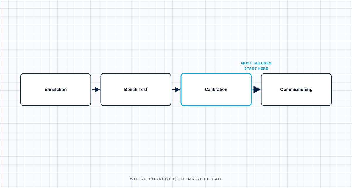
By the time a power electronics program reaches calibration and commissioning, the design has usually already passed simulation, passed design review, and passed initial bench validation. This is exactly why the failures that show up at this stage are the most expensive ones — they aren't design errors in the traditional sense, they're the gap between a model of the system and the actual physical hardware, wiring, and environment it has to operate in. This is a field-level look at where that gap tends to open up, across both EV powertrain electronics and power-electronics.svg)

Current sensor calibration: the drift nobody budgets for

Hall-effect current sensors are calibrated at a reference temperature, usually 25°C, and their offset and gain error both shift with temperature — sometimes significantly, depending on sensor grade. For a traction inverter or a BESS PCS, current sensing accuracy directly drives control loop performance and protection thresholds, and a sensor that's well within spec at room temperature can drift enough at -20°C or +85°C to trip a protection threshold that was set assuming room-temperature accuracy, or worse, fail to trip one that should have.

The practical fix is temperature-compensated calibration — characterizing offset and gain error across the full operating temperature range during production test, not just at one reference point — and it has to be planned into the end-of-line test station from the start, because retrofitting temperature-chamber calibration into a test process designed for room-temperature-only testing is a production line redesign, not a firmware update.

Encoder and resolver calibration for motor control

Position feedback calibration — resolver-to-digital conversion offset, encoder index alignment to motor electrical angle — is one of those steps that looks trivial in a lab with one motor and one inverter, and becomes a genuine production bottleneck at volume, because mechanical tolerance stack-up means every motor-inverter pairing has a slightly different offset that has to be measured and stored, not assumed from a nominal design value.

Two things go wrong repeatedly:

• Calibration procedures validated on engineering-build motors with tighter tolerances than production motors, so the calibration routine's assumptions about acceptable offset range don't hold once production-tolerance parts are on the line, and units start failing calibration that would have passed with the original engineering-build hardware.
• Calibration data storage and traceability — if the calibration offset isn't reliably written to non-volatile memory and linked to the specific motor-inverter serial number pair, a field replacement of either component silently invalidates the calibration, and the resulting control loop instability shows up as an intermittent, hard-to-diagnose field issue rather than an obvious failure.

Hardware-in-the-loop testing before physical integration

HIL testing exists precisely to catch control software behavior against physical hardware dynamics before the actual vehicle or system is available for testing — but its value depends entirely on how faithfully the plant model represents the real system's edge cases, not just its nominal behavior.

The gap that causes trouble later: HIL plant models are usually built and validated against nominal component behavior, and don't always capture component-to-component variation (the same variance discussed in cell qualification and sensor calibration above). A control strategy that's robust against the HIL model's nominal plant but was never tested against the model's parameter tolerance bounds can pass every HIL test and still show marginal behavior on physical hardware that sits at the edge of normal manufacturing variation. Running HIL validation across the actual tolerance envelope of key parameters — not just nominal values — catches this before physical integration, when it's still cheap to fix.

EMC pre-compliance: catching problems before the accredited lab visit

Booking time at an accredited EMC lab for full compliance testing is expensive, and finding a failure there is far more expensive in schedule terms than finding it earlier. Pre-compliance testing with in-house or lower-cost equipment — near-field probing to identify likely radiated emission sources, conducted emissions scanning on power lines — before the formal compliance run consistently pays for itself by turning a "test, fail, redesign, retest at full cost" cycle into a "pre-test, fix, test once and pass" cycle.

The most common late-discovery EMC issue in integrated power electronics is exactly the coupling problem described in 6-in-1 unit design: noise sources and sensitive circuits that were adequately separated on paper but end up close together in the final mechanical layout. Pre-compliance testing on early mechanical samples — not just on bench prototypes with cables laid out for convenience rather than final routing — is what catches this before the accredited lab visit, not after.

Fault injection and functional safety validation

Functional safety validation isn't complete when the normal operating envelope has been tested — it's complete when the system's behavior under fault conditions has been validated against the safety case: sensor failures, communication loss, power supply transients, and combinations of these happening together. Fault injection testing — deliberately forcing failure conditions in a controlled test environment — is how this gets validated, and it's the testing phase most likely to get compressed under schedule pressure because it doesn't demonstrate new functionality, only confirms that failure handling works as designed.

The projects that avoid late functional-safety surprises are the ones that scope fault injection test cases directly from the safety case's assumed failure modes during test planning, not as an afterthought once nominal functional testing is complete and schedule pressure is already building toward a program milestone.

Integration pitfalls: ground loops, shared returns, and bus timing

A handful of integration issues show up so consistently across different projects that they're worth naming directly:

• Ground loops created when a subsystem's chassis ground and signal ground are tied together at more than one point across a wiring harness, creating a circulating current path that injects noise into low-level signals — a classic problem that's easy to prevent with a single-point grounding strategy decided at harness design time, and painful to trace once a vehicle or system is fully integrated.
• Shared return paths where high-current and low-current signals share a return conductor, so switching transients on the high-current path show up as voltage noise on the low-current signal referenced to the same return — common between a traction inverter's power return and a nearby sensor's signal return when harness routing wasn't planned with current path separation in mind.
• CAN bus timing jitter introduced by adding a new node (common when integrating a new subsystem like a BESS EMS into an existing communication architecture) that changes bus loading and arbitration timing in ways that don't show up until the bus is close to saturation — which is exactly when it matters most, during high-message-rate events like fault conditions or dispatch changes.

Commissioning is where the model meets the machine

Every issue in this article shares the same underlying cause: a model — a thermal model, a plant model, a wiring diagram, a safety case — that was correct in its assumptions and incomplete in its coverage of real-world variation. Calibration, integration, and commissioning are the phases where that gap becomes visible, because this is the first point where the actual hardware, with all its manufacturing tolerance, thermal history, and wiring reality, is finally in the loop. Planning test and calibration coverage for that variation from the start — not discovering it during a commissioning window with a schedule already under pressure — is the difference between a program that ships on time and one that doesn't.

FROM FAILURE MODE TO EVIDENCE

01

Define the boundary

Name the operating state, interfaces, tolerances and degraded conditions. A test without a boundary only proves the sample survived once.

02

Capture the right signal

Choose measurements fast and close enough to the mechanism to explain cause, sequence and margin—not just the final alarm.

03

Set a decision rule

Agree before the test what passes, what triggers redesign and what uncertainty requires another experiment.